The Ising model is a simplified description of ferromagnetism where spin-up and spin-down states sit on a d-dimensional lattice with an interaction defined between spins on neighboring sites. In one and two dimensions this model is analytically soluble, but because of that it makes a perfect playground to learn about Markov Chain Monte Carlo methods; a powerful tool with diverse applications in Bayesian statistics, statistical mechanics, and quantum field theory.
Solving the Ising Model in 1D
\[H = -\sum K_{ij}\sigma_i\sigma_j - \mu\sum J_i\sigma_i\] \[Z = \sum_{\{\sigma\}} e^{-\beta H}\]As it turns out we have very nice formulas for energy, specific heat, magnetization, and susceptibility respectively: \(E = -\frac{\partial\ln Z}{\partial \beta}\), \(c_v = k\beta^2 \frac{\partial^2\ln Z}{\partial \beta^2}\), \(M = -\frac{\partial\ln Z}{\partial J} \biggr\rvert_{J=0}\), and \(\chi = -\frac{\partial^2\ln Z}{\partial J^2} \biggr\rvert_{J=0}\)as well as the correlation functions, all in terms of the partition function \(Z\). So, in principle, if we know the partition function, we know everything
The problem is that the number of terms in the sum is exponential in the number of states \(\sigma\). There are two ways to deal with the situation: 1) figure out some fancy tricks to ananlytically coerce this unwieldy beast into submission, or 2) use numerical techniques which exploit the fact that only a relatively small number of states contribute appreciably to the partition function. Here, we’ll do both.
Let’s start with (1):
Let N be the length of the lattice in each direction and assume periodic boundary conditions such that \(\sigma_{N}\) neighbors \(\sigma_{1}\). For simplicity let’s also turn off the external magnetic field (\(h=0\)).
\[Z = \sum_{\{\sigma\}} e^{K\sigma_N \sigma_1} \prod_{k=1}^{N-1} e^{K\sigma_k \sigma_{k+1}}\]Where \(K = \beta J\). Defining the transfer matrix:
\[T_{\sigma_k \sigma_{k+1}} = \begin{bmatrix} e^K & e^{-K} \\ e^{-K} & e^K \\ \end{bmatrix}\]we can rewrite the partition function as follows:
\[Z = \mbox{Tr}T^N = \lambda_1^N + \lambda_2^N\]Diagonalizing \(T\) we find eigenvalues \(\lambda_1 = 2\cosh K\) and \(\lambda_2 = 2\sinh K\)
So we end up with the particularly simple form:
\[Z = (2\cosh K)^N + (2\sinh K)^N\]Thermodynamic Limit
The abrubt changes in thermodynamic properties observed in phase transitions appears to be at odds with a description in terms of analytic functions. After all, the partition function is nothing more than a finite sum of exponentials.
Being that \(e^x\) is everywhere analytic and realizing that a finite sum of analytic functions is itself analytic the partition function might at first seem hopelessly incapable of describing the physics of phase transitions. But critically (what a pun!), an infinite sum of analytic functions need not be analytic. A familiar example comes from Fourier Series where we find that an infinite number of sine waves can add up to a square wave:
Typically we are not interested in small lattice sizes and want to know what the behavior looks like in macroscopic systems. Defining an intrinsic quantity \(\,f = \frac{1}{N\beta}\ln Z\) called the free energy per spin, we can take a well-defined limit as the number of sites goes to infinity. For our 1D solution:
\[\lim_{N \rightarrow \infty}f = \ln2 + \ln \cosh K\]Which is completely smooth. No phase transition in 1D. It seems we’ll have to try something more complicated if we are to capture our elusive prey.
Criticality in 2D
The full solution in two dimensions is very complicated to derive (apparently it took Richard Feynman 14 pages to explain it in his lectures on statistical mechanics). I won’t endeavor to try your patience to such an extent, but fortunately we can find the critical temperature in a slightly less painful manner, using a result called Kramers-Wannier Duality. Nevertheless, a certain amount of pain must be endured, so if you’re more algorithmically minded feel free to make a cowardly break for the next section.
To begin we rewrite the partition function as
\[Z = \cosh(K)^N Z^\prime\] \[Z^\prime = \sum_{\{\sigma\}} \prod_{\langle i,j \rangle} [1 + \sigma_i \sigma_j \tanh(K)]\]using the fact that \(e^{\pm x} = \cosh(x)[1 \pm \tanh(x)]\). We can keep track of the terms combinitorically by matching the \(\sigma_i \sigma_j \tanh(K)\) terms up to edges in a subgraph \(P\) of the lattice:
\[Z^\prime = \sum_{\{P\}} \prod_{\langle i,j \rangle \in P} \sigma_i \sigma_j tanh(K)\]Consider a subgraph consisting of a single non-self-intersecting path and let \(P(k)\) denote the \(k\)th site along the path:
unless \(P(0) = P(L)\), i.e.: \(P\) is a closed path. More generally, we can use this same idea to prove that the only link configurations that contribute to the partition function are those that form even subgraphs. Using this fact we can further simplify \(Z^\prime\):
\[Z^\prime = \sum_{l=0}^{2S} c(l) \tanh(K)^l\]where \(c(l)\) counts the number of even subgraphs with length \(l\). This is one half of the duality, usually referred to as the high temperature expansion.
Now, consider the dual lattice whose sites sit in the squares of the original lattice and whose neighbors are those squares it shares an edge with. When we use periodic boundary conditions the lattice forms a torus, and in fact the dual lattice forms an identical torus!
Given an even subgraph on the original lattice there exists a two-to-one correspondence with spin configurations on the dual lattice:
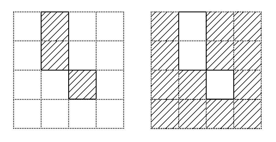
At least, that is almost true. In fact the correspondence breaks down for certain subgraphs which wrap completely around the torus, but these terms contribute negligbly to the summation and will go to zero in the thermodynamic limit.
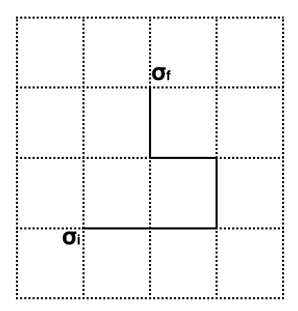
At low energy all of the spins in the dual lattice will be lined up, so the ground state energy is \(H_0 = -KN\). Thus, we can rewrite the original Hamiltonian as:
\[H = H_0 + \sum_{\sigma_i \neq \sigma_j \vert \langle i,j \rangle} 2K\]Here the summation is only over the links connecting sites of differing spin, which occur precisely across each of the edges present in the subgraphs of the high temperature expansion; each edge lifing the energy by \(2K\). Note that the energy of a configuration again depends only on the number of edges in the subgraph. This allows us to write the partition function in a suggestively familiar form:
\[\hat{Z} = 2e^{\hat{K}N}\sum_{l=0}^{2N} c(l)e^{-2\hat{K}l}\]where the factor of 2 out front comes from the two-to-one correspondence between the dual lattice and even subgraphs on the original lattice. Behold: the low temperature expansion!
As we take \(N \rightarrow \infty\) both expansions must be identical under the identification \(\tanh(K) \leftrightarrow e^{-2\hat{K}}\):
\[\frac{\hat{Z}}{2e^{\hat{K}N}} = \frac{Z}{\cosh(K)^N} = \sum_{l} c(l)e^{-2\hat{K}l} = \sum_{l} c(l) \tanh(K)^l\]This identification defines a mapping between high temperature and low temperature which preserves analytic behavior. Since critical points are defined by nonanalyticity, critical points must be mapped to critical points.
If we assume the system contains only one phase transition, it must be mapped to itself. Thus \(K_c\) occurs when \(K=\hat{K}\), and manipulating the tanh term we get a polynomial in \(\chi = e^{2K_c}\):
\[\chi^2 - 2\chi - 1 = 0\]Solving this we find the critical temperature
\[T_c = \frac{2J}{k \ln(1+\sqrt2)}\]and can now go to sleep. . .But ho! I am not through with you yet:
The Metropolis Algorithm
Every physics treatment of this algorithm that I’ve read feels as if it’s described backwards, so I’m going to try doing things a bit differently.
The overall idea is to build a markov chain whose equilibrium distribution of states matches the partition function. Let \(P\) denote the \(2^N\times2^N\) transition matrix whose entries \(P_{AB}\) represent the probability of transitioning from state \(A\) to state \(B\).
A sufficient, but not necessary, condition for the Markov chain to be in equilibrium is for it to satisfy the detailed balance condition:
\[\pi_A P_{AB} = \pi_B P_{BA}\]where \(\pi\) is the probability distribution over states. Since we want \(\pi\) to give the partition function, we must have \(\pi_A = \frac{1}{Z}e^{-\beta E_A}\). Thus:
\[\frac{\pi_A}{\pi_B} = \frac{P_{BA}}{P_{AB}} = e^{\beta[E_B-E_A]}\]We have some freedom in choosing transition probabilities, they just need to satisfy this equation. So let’s define:
\[P_{AB} = \frac{1}{N} \mathcal{A}_{AB}\] \[\mathcal{A}_{AB} = \left\{ \begin{array}{lr} e^{\beta[E_B-E_A]} & : B < A\\ 1 & : otherwise \end{array} \right.\]for \(A \neq B\) being nearest neighbors and \(0\) otherwise. Finally, the requirement that \(P\) be a stochastic matrix fixes \(P_{AA} = 1 - \sum_{B \neq A}P_{AB}\).
Now that we know all this, we can finally define the Metropolis Algorithm:
- initialize lattice with some spin configuration \(\{\sigma\}\)
- choose \(\sigma_i\) uniformly at random (drawing from \(p(\sigma_i) = \frac{1}{N}\))
- set \(\sigma_i := - \sigma_i\) defining the transition \(A \rightarrow B\)
- accept new state with probability \(\mathcal{A}_{AB}\)
- if new state is rejected reset \(\sigma_i\) to its previous state
- proceed to step (1)
Since the algorithm initializes the spins in an arbitrary configuration there is a certain thermalization time needed before the system actually reaches equilibrium. Once equilibrium is reached we can treat subsequent states as draws from the partition function. We will generally want each draw to be independent from the previous draw. To achieve this we can simply experiment to find a fixed number of iterations between draws for which the correlations are sufficiently close to zero.
A Curious Link to Quantum Field Theory
The starting point for most quantum field theory is the path integral, such as this one describing a real scalar field:
\[Z = \int \mathcal{D}\phi e^{\frac{i}{h}\int dx^4 [\frac{1}{2}\partial_\mu\phi\partial^\mu\phi - \frac{1}{2}m^2\phi^2 - V(\phi)]}\]Fancifully put, a real scalar field is just the physics in the continuum limit of an infinitely large mattress.
The path integral is essentially a sum over all paths in spacetime. The notation of \(\partial_\mu\phi\partial^\mu\phi\) with one index raised and one lowered encodes the metric of Minkowski space. Described using this geometry the physics of special relativity essentially all boils down to the fact that you can convert space and time into each other by rotating through an imaginary angle.
Since the functions being described here are analytic we can rotate into imaginary time to do our calculations in euclidean space and then use analytic continuation to put our results back into ordinary spacetime.
But when you rotate into Euclidean space the exponent gets shuffled around:
\[Z = \int \mathcal{D}\phi e^{-\frac{1}{\hbar}\int dx^4 [\frac{1}{2}\delta^{\mu\nu}\partial_\mu\phi\partial_\nu\phi + \frac{1}{2}m^2\phi^2 + V(\phi)]} = \int \mathcal{D}\phi e^{-\frac{1}{\hbar} H[\phi]}\]If you identify \(\beta \leftrightarrow 1/\hbar\) this is exactly analogous to the partition function in statistical mechanics. This is an example of a duality: every problem in quantum field theory has a corresponding problem in statistical mechanics, and vice versa. This greatly expands the variety of techniques at our disposal and has proven to be a powerful tool in physics. In particular the MCMC simulation we used here can be applied to quantum field theories and has been critical to understanding the nonperturbative aspects of quantum chromodynamics. But that’s for a future post…
Links and Resources
[2] Stanford Handout on the Ising Model
[3] The Renormalization Group for Ising Spins
[4] More Renormalization Group Methods