Understanding Similarity With Markov Chains

Facebook is a graph. Twitter is a graph. The internet is a graph. Almost any other kind of data you can think of probably has some sort of graph structure if you squint kinda funny and look at it from the right angle. So if you’re a data scientist, it’s pretty important to know how to deal with graphs. It’s a common question to ask how one can find things that are similar in a graph, but finding a good answer may not be as simple as you think.

Shortest Path

Starting off with a simple first guess we could choose to measure similarity by the shortest path connecting two nodes. In some ways this makes a lot of sense, particularly if you start thinking about your data as lying on some kind of submanifold in feature space (which you tend to do if you have an affinity for differential geometry). As it turns out, as the number of datapoints sampled from this hypothetical distribution goes to infinity you can meaningfully talk about the shortest path distance converging to the distance along a geodesic in the data manifold.

Cool. But for certain types of graphs and applications this might not be good enough, and many naturally occurring graphs such as social networks and link graphs have degree distributions which roughly follow a power law:

for some constant $\gamma$. Most vertices will have small degree, but the presence of vertices which connect to a substantial proportion of \(\{v\}\) enables even the most disparate vertices to be connected by a short sequence of hops. This phenomena is well exemplified by the “Six degrees of Kevin Bacon” game.

Markov Chains

The picture to have in your head when you think about Markov Chains is just a (possibly directed) graph where every node’s outgoing edge weights sum to one and so can be interpreted as probabilities.

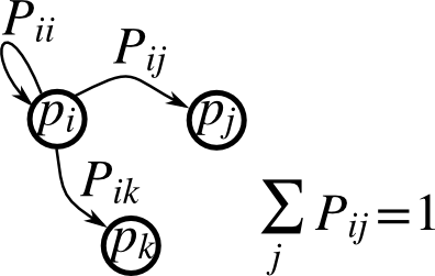
Given any weighted graph we can always normalize the edge weights to satisfy this condition:

where W is the weight matrix of the original graph, and D is a diagonal matrix defined by \(D_{ii} = \sum_j W_{ij}\)

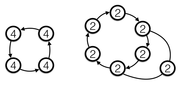
Starting at any vertex we can generate a random walk by repeatedly choosing a new vertex to move to according to the transition probabilities \(P_{ij}\) for the edge leaving i and arriving at j. A Markov Chain is said to be ergodic if (I) given any two states i and f there exists a path from i to f that can be traversed with nonzero probability, and (II) every state is aperiodic. Note, the Markov chain above is not ergodic because it fails condition (I): you get trapped in either states j or k and can’t make your way back to the other states. I won’t rigorously define what periodicity is meant here because wikipedia does a good enough job and this article is long enough as it is, but below are a couple of simple examples in which every state is periodic, with the periodicity of each state labeled:

Consider a vector \(\pi\) which represents a probability distribution over each of the vertices. If we start with all of the probability mass centered on one vertex and iterate the distribution according to

then in fact this is the random walk we just described. More generally we can start with any initial distribution and we’ll end up with a kind of weighted average over random walks with different starting points.

A distribution \(\pi_0\) is called an equilibrium distribution if it satisfies:

What do Random Walks Give us that Shortest Paths Don’t?

Consider a vertex i adjacent to a high degree vertex j, and a vertex k which has i as its only neighbor. Intuitively, it should make sense that \(Sim(j, i) > Sim(i, k)\) because their association is more uniquely distinguishing, but under path similarity they are the same.

Consider a random walk starting at i. If it hops to vertex j then at the next step the probability distribution would get smeared out over every vertex that j is connected to, so ultimately j will tend to end up with a low probability. Conversely, if the random walk hops over to k, then at the next step the only choice is for it to come back to i. In other words, the random walk can tell that there’s less randomness associated with these connections!

It’s possible to define a variety of different notions of similarity based on Markov chains, but they basically all capture this key feature. There’s no clear way to say which is theoretically best, and if you have time it might be advisable to try several of them out and compare their performance on your particular data.

Below I discuss some possible choices, how to compute them, and some of their important properties.

PageRank

We can compute the personalized PageRank for some initial distribution via a power iteration as follows:

from scipy import sparse


# pi0 is any initial distribution
def personalizedPageRank(W, pi0, beta=.1, n=30):
	D_inv = sparse.dia_matrix(W.shape)
	D_inv.setdiag([(not num or num**-1+1)-1 for num in W.sum(axis=0).tolist()[0]])
	P = D_inv*W

	pi_n = pi0.copy()
	for i in range(n):
		pi_n = beta*pi0 + (1-beta)*pi_n*P

	return pi_n

If you don’t need or want a symmetric notion of similarity then this might be enough: given \(\pi_0\) centered on vertex \(v\) you compute the PageRank and you take the vertices assigned the highest probability as the most similar.

Alternatively, given any two vertices, we compute their PageRank’s separately, so each vertex gets transformed into a probability distribution. Now we simply use some standard method for comparing probability distributions such as KL Divergence (which is also non-symmetric) or Bhattacharyya distance (which is symmetric).

Commute Times and Hitting Times

Hitting times are a very interesting property that can capture a considerable amount of the connectivity structure of a graph. But depending on our application they might not map to the notion of similariy we want because it’s not symmetric between vertices, i.e.: the hitting time from a to b is not the same as the hitting time from b to a. Fortunately there a very easy way to fix this: define the commute time \(C_{ij} \equiv h_{ij} + h_{ji}\) as the expected time to travel from i to j and then return back to i.

Great! Now that we have a nice, symmetric notion of Markov similarity, how do we compute it?

where \(L^\dagger = (L^T L)^{-1}L^T\) is the Moore-Penrose pseudoinverse, \(L = I - D^{-1/2} W D^{-1/2}\) is the normalized graph Laplacian, and \(\pi\) is the stationary distribution of \(P\). Now personally, I think this is a very cool formula. The only problem is that it’s totally useless for most practical calculations. Assuming the graph we’re dealing with is large enough to require exploiting its sparsity we’re out of luck because this formula relies entirely on computing the inverse of a very large, sparse matrix. And generically the inverse of a sparse matrix will be dense.

This would seem to put us in a difficult position, but fear not brave programmer, for all hope is not lost!

Power Iteration

The hitting time can be computed by the following expectation value:

Truncating this series at some \(T-1\) and adding in a remainder term we get the truncated hitting time:

Finally, we can rewrite the above equation as follows to avoid having to compute powers of the transition matrix:

This approximation will always underestimate the true hitting time, as all the unused probabily mass after \(T-1\) gets lumped into the \(T\) term. Thus we’ll have to play with cutoff to make sure the range \([0, T]\) has sufficient resolution to capture most of the interesting behavior.

from scipy import sparse


def truncatedHittingTimes(W, i, T=100):
	D_inv = sparse.dia_matrix(W.shape)
	D_inv.setdiag([(not num or num**-1+1)-1 for num in W.sum(axis=0).tolist()[0]])
	P = D_inv*W

	one_vector = np.ones(P.shape[0])
	h = np.zeros(P.shape[0])
	rho_t = np.zeros(P.shape[0])
	used_probability = np.zeros(P.shape[0])

	rho_t[i] = 1
	used_probability[i] = 1

	for t in range(1, T):
		rho_t = rho_t*P
		currentProbability = rho_t*(one_vector-used_probability)
		used_probability += currentProbability
		h += t*currentProbability

	return h + T*(one_vector-used_probability)

Coda

This still isn’t the end of the story, as e.g. Luxburg et al. 2011 study the behavior of commute times in certain types of random graph and prove that as the size of these graphs tends to infinity the commute times converge to purely local quantities with respect to the considered vertices. Thus for such graphs commute times may fail to convey any meaninful information as a distance measure! Diffusion distance could be a good alternative if you’re faced with this situation, but there’s an important moral here: much like machine learning algorithms there’s no free lunch when it comes to measuring distance on graphs. Always think about the failure cases and never try just one.

Links and Resources

D. Rao, D. Yarowsky, C. Callison-Burch, Affinity Measures based on the Graph Laplacian.

U. Luxburg, A. Radl, M. Hein, Hitting and Commute Times in Large Random Neighborhood Graphs.